
VISUAL INTERPRETATION OF STOCK PREDICTION USING SENTIMENT ANALYSIS
Abstract
Stock trading is an activity of buying and selling stocks of an organization and the its market plays a considerable role in the growth of a country’s economy. It is directly related to the commerce and industries that a nation possesses. The market is not only a source of funds for an organization but also acts as a platform for stock traders and individual owners to buy and sell stocks. For these end users making the buy/sell decisions is a big deal. So, the stockbrokers, traders, business analysts, end users have their own trading rules, do planning, set entry and exit rules, use technology etc. as they are very much required to keep the losses to a minimum. There are several factors which effect daily stock prices of an organization among which the news headlines relating to the organization play a significant role in price fluctuations. These news headlines create a sentiment towards the organization among the users and effect these prices. This model taken in the news headlines relating to an organization and returns a sentiment value for predicting the next days stock price changes. All the findings of the model are presented through several graphs and tables for the end user to better understand the findings.
Introduction
Stock markets can play a pivotal role in stabilizing the economies on a global scale by avoiding the repercussions of a recession by evading the potential bankruptcy of companies and loss of billions for the investors and shareholders and thus avoiding the collapse of stock markets(“Importance of stock market”,n.d.). The stockholders and traders follow many approaches and strategies to make better trading decisions.
Trading plan involves the prerequisites that one needs to have before planning anything in general. One needs to know the terminology, the nitty-gritty of the trading market. One must also know the reasoning behind the past gains or losses. Planning needs analyzing the situation and then a plan to deal with it.
Capital investment and protection. To start a trade the first step is to introduce the capital. Accumulation of it must have involved a lot of savings and effort along with time. One needs to be very vigilant as the losses can be to the extent of getting bankrupted. (folger j,2019)
The stock traders must be focused on learning more each day. Focused observation, analysis of the stock market trends are prerequisites. The nature of stock markets is very dynamic meaning that it depends on several factors including world politics, events, economies, oil supply/demand, world leader ideologies and even the weather.
Risking wisely. Risk must only be taken if you can afford to lose. The assets used for trading must be expendable and not be allotted for any other purposes. Because losing money can be traumatic.
The trading decisions must be made based on facts. We can always research regarding, on internet. And the risks of this could be internet thefts and false sources. One must know the Genuity of information and its sources.
It is also advisable to always reevaluate your trading plan due to the sudden stock market fluctuations and changing trends. It is also very important to put trading in perspective. That is one must not totally indulge their emotions with trade wins/losses. This will facilitate for a healthy stock trading.
Utilization of technology. Technology utilization is having the know-hows of viewing and analyzing the markets through internet. Getting updates through smart phones allows us to monitor trade prices, equities, bonds etc. virtually from anywhere. As discussed earlier the economy of most of the countries is dependent on the stock market trading, it has the potential to uplift the economy and collapse. Many machine learning technologies are now being used to predict the stock prices. Out of the many factors responsible for the stock price changes social media is playing a significant role. The news relating to an organization or the opinions/discussions held on twitter are playing a role in forming a biased view towards an organization. This may have a fair amount of effect on an organizations stock price. For example, the news of Steve jobs’s death. Here the investor will be in the fear of investing in the apple stocks so for a few days stocks for Apple Inc may be decrease in value . Another one, the headlines can directly affect the stock price of next day like US banning Huawei phones completely. This will affect next day stock price of Huawei people will be willing to sell the stock.
In this project I have taken up the new headlines relating to apple company and tried to predict the organizations future stock price changes through sentiment analysis.
Modules
Data Downloading
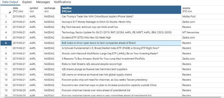
The headlines regarding a company are downloaded every day and stored in the database. the psycopg2 api is used to set up a connection to the dbms. These headlines are downloaded from the Finviz and Nasdaq news websites. The postgres database management systems is used to store the data. This project is developed using the headlines from April 1st to June 27th, 2019. By going through Nasdaq news website the data taken is changed into month-date-year format (from month-date-year). The required data is crawled through web and is stored as a dataframe in the database. This dataframe has the following fields: date, name(organization), exchange(Nasdaq), source(news websites), headlines. Here is the table that represents this dataframe:
Data Preprocessing
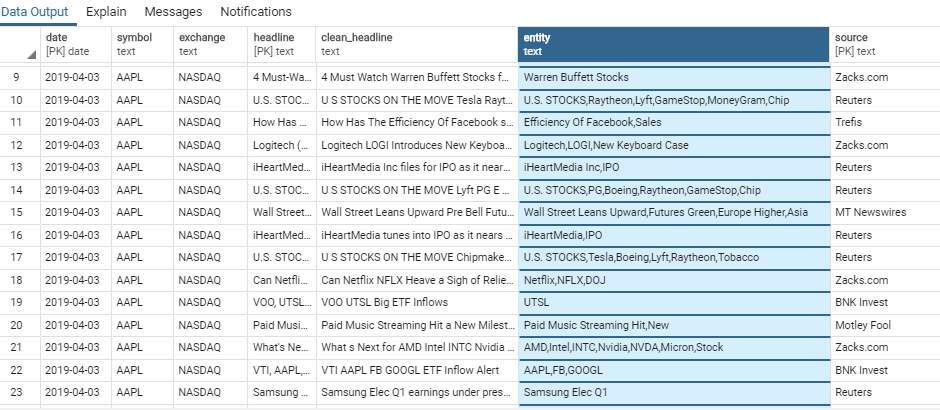
The headlines that are obtained from the news websites are preprocessed by removing special characters and numbers. It also contains a get_continuous_chunks(text) method which initially splits off the words in the sentence with its punctuation using word_tokenize() of nltk library. These words are then tagged with its parts of speech with the help of pos_tag(). The output of this is then passed onto the ne_chunk() which groups them into chunks. Tree functionality of nltk then represents them into a hierarchical grouping of leaves and sub trees. This method will return the entities that are present in each headline. this will facilitate for the user to easily search and identify for a headline by using the entities instead of skimming through the whole bunch of data. The dataframe representing the output of this function is stored in this way.
Getting Polarity
So, polarity for each headline is generated using one of the three methods(simple polarity, textblob or Vader).
In simple polarity, sentiment classification is done with Liu and Hu opinion lexicon. This function counts the number of positive, neutral and negative words in a sentence and classifies it on the basis of polarity of the headline. Words that are not in the lexicon are considered as neutral.(Pantane,n.d.)
def get_simple_polarity(sentence):
tokenizer = nltk.tokenize.treebank.TreebankWordTokenizer()
pos_words = 0
neg_words = 0
neutral = 0
tokenized_sent = [word.lower() for word in tokenizer.tokenize(sentence)]
if len(tokenized_sent) == 0:
return 0
opinion_lexicon = nltk.corpus.opinion_lexicon
for word in tokenized_sent:
if word in opinion_lexicon.positive():
pos_words += 1
elif word in opinion_lexicon.negative():
neg_words += 1
else:
neutral += 1
total_words = pos_words + neg_words + neutral
polarity = (pos_words – neg_words)/total_words
return polarity
Textblob polarity is a predefined functionality for sentiment analysis which provides with the polarity of the input data. It returns polarity values in the intervals of [-1,1]. Negative value means a negative emotion and vice versa. Textblob for sentiment analysis also returns subjectivity of the sentence along with the polarity. Subjectivity lies in the interval of [0,1] where it represents whether the input sentence passed is not a factual information. Here we only use the polarity that the function returns. Textblob not only is used for sentiment analysis but also does Words Inflection, Lemmatization, Ngrams, tagging parts of speech, noun phrase extraction etc.
def get_textblob_polarity(sentence):
analysis = textblob.TextBlob(sentence)
return analysis.sentiment.polarity
Vader
Vader stands for Valence Aware Dictionary and Sentiment Reasoner which is a python package used for sentiment analysis. It is considered great for calculating sentiment values for social media content and generates four metrics(positive, negative, neutral and compound) for the words that match with the lexicons present with the package.
def get_vader_polarity(sentence):
vader_analyzer = nltk.sentiment.SentimentIntensityAnalyzer()
vader_polarity = vader_analyzer.polarity_scores(sentence)
polarity = 0
pos = “pos”
neg = “neg”
if vader_polarity[pos] > vader_polarity[neg]:
polarity = vader_polarity[pos]
elif vader_polarity[pos] < vader_polarity[neg]:
polarity = vader_polarity[neg] * -1
return polarity
The final polarity of the headline is considered as the value returned by the Vader functionality. If this value is zero, then textblob’s polarity is considered. If this polarity is also zero, then only the simple polarity is taken into consideration for the final polarity.
if vader_polarity[pos] > vader_polarity[neg]:
review = vader_polarity[pos]
elif vader_polarity[pos] < vader_polarity[neg]:
review = vader_polarity[neg] * -1
else:
if blob_polarity == 0:
review = simple_polarity
else:
review = blob_polarity
return review
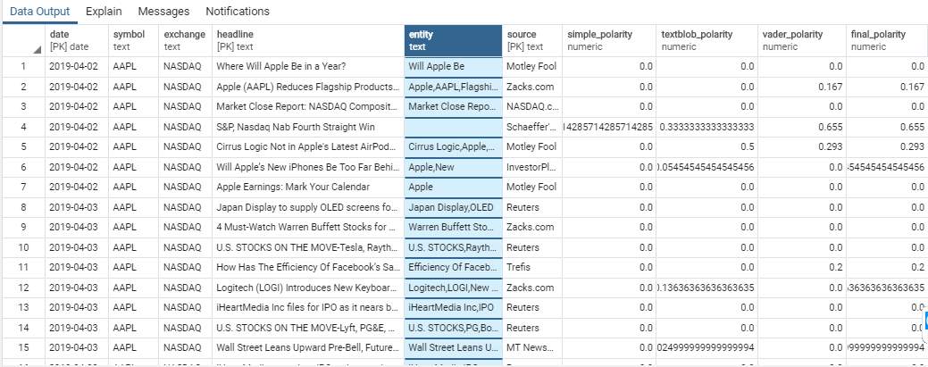
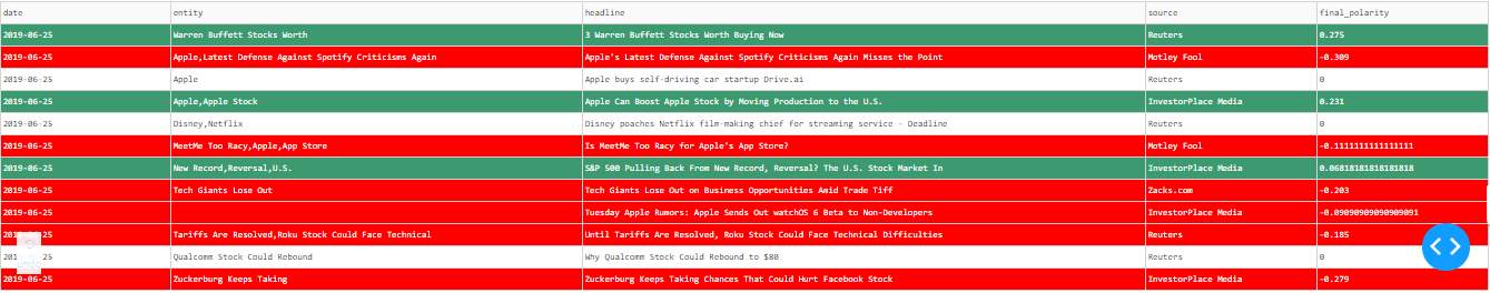
This table in the database represents the headlines with all the values of polarities obtained along with the finally considered polarity value.
Generating Sentiment Values
Basically, the function that calculates the sentiment for that day considers three parameters. One is the polarity of the present day then is the previous days sentiment value where day depends on which weekday it is, and the third parameter is the todays date. If it is not a Sunday, then its previous sentiment value will be the sentiment of the previous day. For example, if you want to calculate the sentiment of Monday then your previous sentiment will be of Sunday. If you want to calculate the sentiment of Sunday, then polarity of three days that is Friday Saturday and Sunday are considered. And the previous days sentiment will be the sentiment of Thursday. The reason for this is that the stock market is closed on weekends i.e. Saturday and Sunday. So, while predicting stock price changes for Monday, the headlines on Friday, Saturday and Sunday are considered.
Get Help With Your Essay
If you need assistance with writing your essay, our professional essay writing service is here to help!
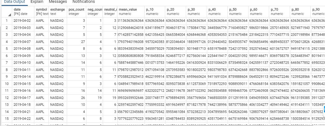
The recent polarity obtained is taken and the count of the positive, negative and neutral is stored in respective variables( pos_count, neg_count, neutral_count). The mean of these count variables is taken. For the neutral polarities to not normalize the mean they are not considered. If mean by any chance is not a number, then it is assigned a value of 0.
By using the EMA(Exponential Moving averages) method we calculate 10 sentiment values by giving varying weightages to previous sentiment and the mean we procured. the tenth value will be the mean calculated. The alpha value varies from 0 to 1 in the intervals of 0.1. The formula used is given below:
ema = (1-alpha) * prev_sentiment + alpha * todays mean_value
final_df[‘p_10’] = 0.9 * sentiment_df[‘p_10’] + 0.1 * mean_value
In the above statement the previous sentiment is given a higher weightage which depict the long-term effects of a news headline on present stock prices.
Similarly
final_df[‘p_90’] = 0.1 * sentiment_df[‘p_90’] + 0.9 * mean_value
gives more importance to present day news headlines than the previous news.
The average of all such values is taken and that is the sentiment for that day.
Result Evaluation
This program recommends whether to buy or sell a stock by generating buy, sell, strong buy and strong sell signals. A strong buy or strong sell signal is generated if the buy or sell percentages exceed or equals to 80%.the other cases are explained below with appropriate code. Even the intraday predictions are done. In intraday stock exchanges a stockholder wants to buy and sell the stock on almost the same day to incur small profits on the stock.
The recommendation value for a weekday is stored in its previous day’s recommendation value. For example, the recommendation for Wednesday is given by the recommendation value of Tuesday.
First, the stock prices of that day are stored into the database to get the close-open value which also helps determine the next day’s recommendation. The previous sentiment information for that day is extracted from the database. The tenth value is the mean value which considers only todays polarity not yesterday’s sentiment. the following conditions are considered to initially generate the buy/sell signals:
for i in range(6,16):
if rows[i] > 0 and change > 0 :
result.append(“buy”)
elif rows[i] > 0 and change < 0:
result.append(“buy”)
if rows[i] < 0 and change < 0 :
result.append(“sell”)
elif rows[i] < 0 and change > 0:
result.append(“sell”)
Here the rows[i] take the values from mean,p_10,p_20,p_30,…p_90. The above conditions are explained below:
- if sentiment value is positive and change in stock price is positive then buy signal is generated because the sentiment value favors the stocks and there already has been an increase in price the previous day.
- if sentiment value is positive and change in stock price is negative then buy signal is generated as the sentiment is in favor and stock price has decreased which further decreases the cost price.
- if sentiment value is negative and change in stock price is positive then sell signal is generated. As the stock you have may lose its price the next day and the change on that day positive indicating increase in stock that day.
- if sentiment value is negative and change in stock price is negative then sell signal is generated. The reason for this being that the stock has already decreased in value and on further delay would decrease it value furthermore.
A percentage of these buy/sell signals is calculated.
buy_percent = (int(result_dict[‘buy’])/10) * 100
sell_percent = (int(result_dict[‘sell’])/10) * 100
Then the following conditions are given to generate the final strong buy/sell, buy, sell signals for the next day.
if buy_percent >= 80.0:
final_prediction = ‘Strong Buy’
As the buy percentage is greater than or equal to 80% a strong buy signal is generated.
elif buy_percent < 80.0 and buy_percent > sell_percent:
final_prediction = ‘Buy’
A buy signal is generated as the buy percentage being less than 80 is still greater than the sell percentage for that day.
elif sell_percent >= 80.0:
final_prediction = ‘Strong Sell’
As the sell percentage is greater or equals 80%.
elif sell_percent < 80.0 and sell_percent > buy_percent:
final_prediction = ‘Sell’
a sell signal is generated as the sell percentage being less than 80 is still greater than the buy percentage for that day.
elif sell_percent == buy_percent:
final_prediction = “Hold”
hold signal also exists in cases where the buy and sell percentages are equal.
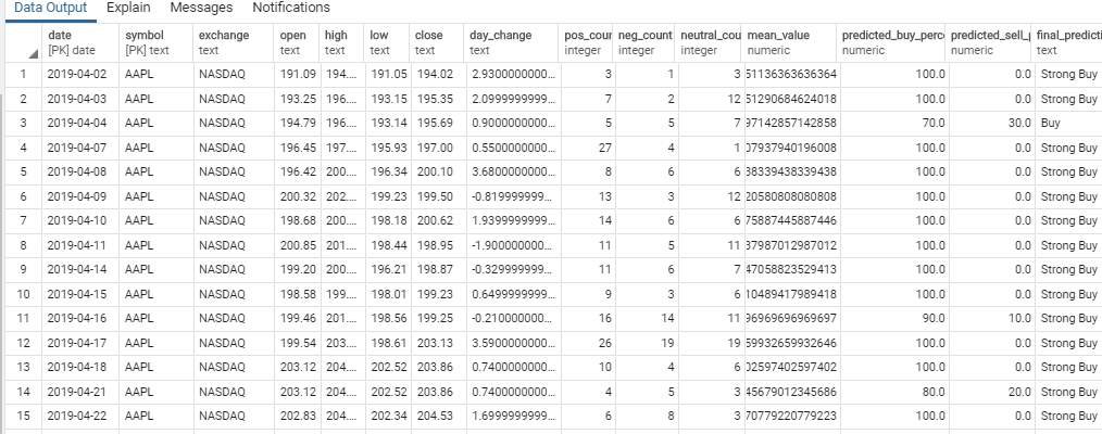
A dataframe with the values date, symbol, exchange, open, high, low, close, change, mean, positive_count, negative_count, neutral_count, buy percentage, sell percentage and final prediction is stored into the database.
generate_result_summary(date, stock_df, recommendation_df)
This method determines whether the recommendation for that day was accurate or not even for intraday stock trading. For this it needs the actual stock prices of that day.
For interday stock prediction accuracy it compares final prediction and (close-open) values. If the final prediction is buy or strong buy and the difference(close-open) is positive than our prediction is correct else wrong.
final_prediction == ‘Buy’ :
if close_open_change > 0:
result_interday = ‘Correct’
else:
result_interday = ‘Wrong’
And
final_prediction == ‘Strong Buy’ :
if close_open_change > 0:
result_interday = ‘Correct’
else:
result_interday = ‘Wrong’
If the final prediction is sell or strong sell and the difference(close-open) is negative than our prediction is correct else wrong.
elif final_prediction == ‘Sell’ :
if close_open_change < 0:
result_interday = ‘Correct’
else:
result_interday = ‘Wrong’
elif final_prediction == ‘Strong Sell’ :
if close_open_change < 0:
result_interday = ‘Correct’
else:
result_interday = ‘Wrong’
For intraday prediction accuracy,
The final prediction is compared with difference between high/low and open prices.
The final dataframe with all the new values is stored into the database as below:
Result_headline.py
This program checks for the accuracy of the prediction made by considering the actual stock prices that are released when the stock market is closed for the day.
The counts of rightly and wrongly predicted values is taken, and percentage is taken.
correct_interday = len(df.loc[df[‘result_interday’] == ‘Correct’])
wrong_interday = len(df.loc[df[‘result_interday’] == ‘Wrong’])
total_interday = correct_interday + wrong_interday
accuracy_interday = (correct_interday/total_interday) * 100
correct_intraday = len(df.loc[df[‘result_intraday’] == ‘Correct’])
wrong_intraday = len(df.loc[df[‘result_intraday’] == ‘Wrong’])
total_intraday = correct_intraday + wrong_intraday
accuracy_intraday = (correct_intraday/total_intraday) * 100
The accuracy thus obtained for this project for interday prediction is 50% and intraday is 54.545454%
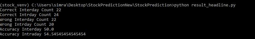
Dashboard.py
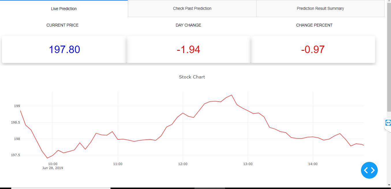
I have programmed a dashboard using dash components in python to represent the results of the project. It contains tabs with livestock prices, pie chart, donut chart, bar graph and tables containing various findings.
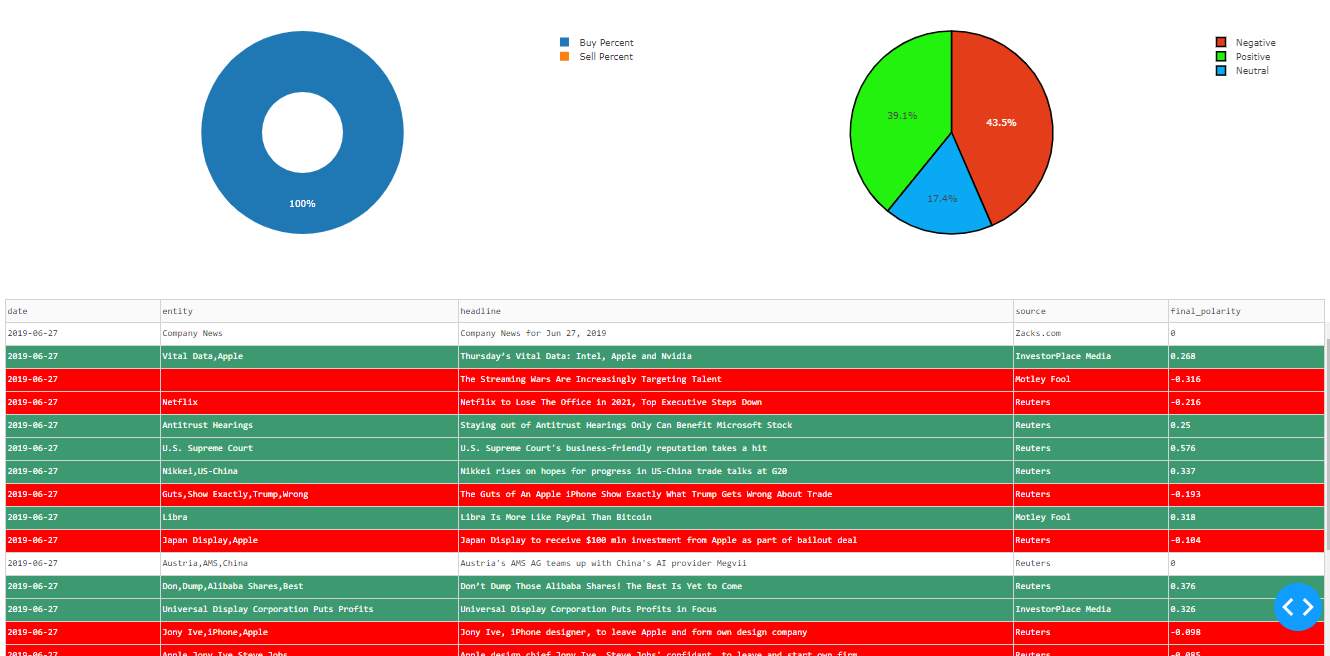
The live prediction tab has the livestock prices that are represented with a line graph which gets updated after every five minutes. This tab also has a donut chart representing the buy and sell percentages for that day. Alongside this chart is the pie chart which represents the total number of positive, negative and neutral headlines percentage. The table at last represents the headlines with the polarity generated for them.
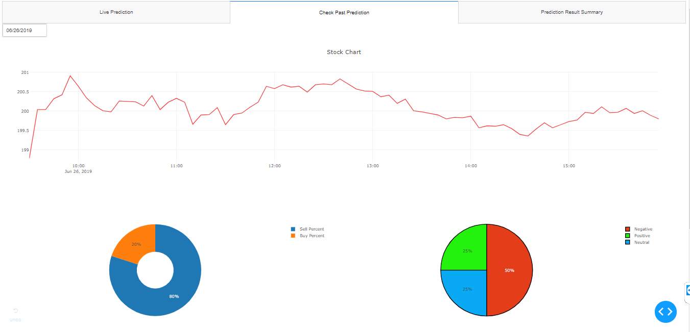
The next tab represents the past day prediction details with the stock prices for time intervals of that day as a line graph. The donut and the pie charts represent the values of the past day.
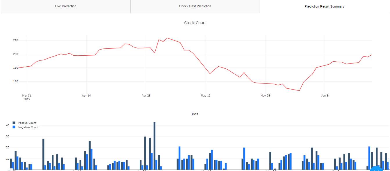
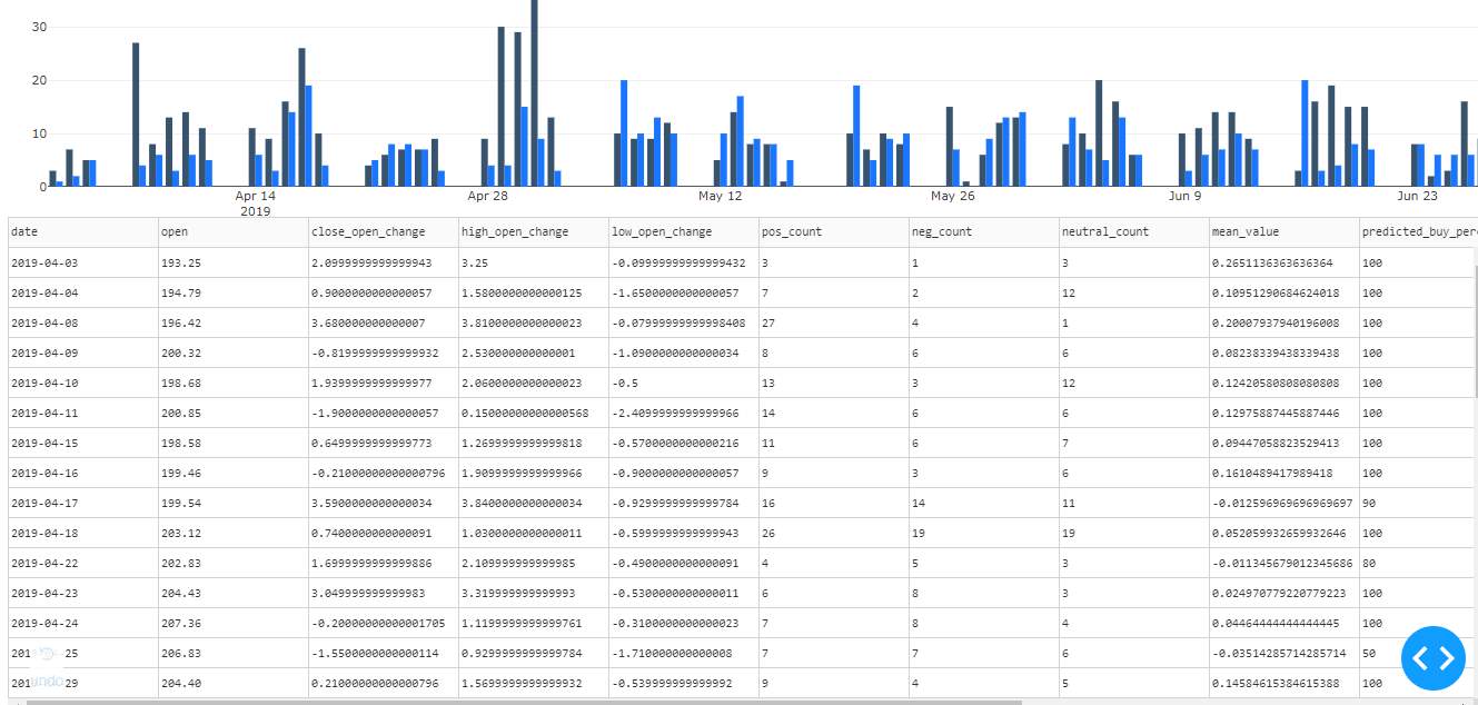
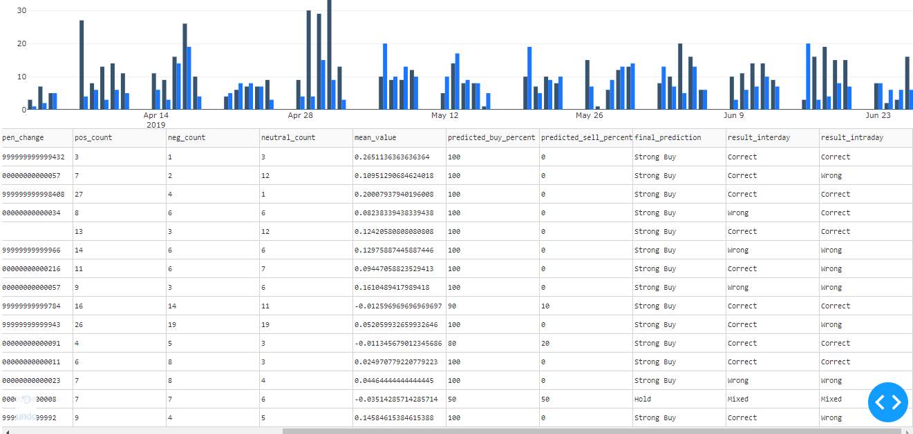
The final tab is the prediction summary tab which represents the prediction information we have done so far. It had a line graph representing the stock prices and their close prices. The double vertical bar graph represents the positive and negative counts of all the days. The table at last represents the complete prediction and result summary.
Conclusion and Future Scope
With more and more advancements in machine learning techniques used for stock price change predictions, several distant factors effecting the stock market are able to be traced for a better control over an individual’s financial investments. Also the information about the major and minor incidents relating to an organization its relation with the organizations financial value can be thus established.
I would further like to increase the accuracy obtained from this project by implementing nuances of procedures and API’s for generating sentiment for the headlines.
As we are using only the headlines for this prediction, another scope would be to increase the domain by giving the news articles also as input for analysis.
Working code
Download_headline_data.py
import requests
import pandas as pd
import psycopg2
from scrapy.selector import Selector
import datetime
“””Get Historic headliens using finviz”””
def get_daily_headlines_data(symbol, number_of_days):
final_df = pd.DataFrame()
url = ‘https://finviz.com/quote.ashx?t=’ + symbol
page = requests.get(url)
sel = Selector(text=page.content)
times = sel.xpath(‘//table[contains(@id,”news-table”)]/tr/td/text()’).extract()
headlines = sel.xpath(‘//table[contains(@id,”news-table”)]/tr/td/a/text()’).extract()
sources = sel.xpath(‘//table[contains(@id,”news-table”)]/tr/td/span/text()’).extract()
times = [x.strip() for x in times if x.strip()!=”]
head_len = len(headlines)
count = 0
for i in range(0,head_len):
if len(times[i]) > 10:
count += 1
headline_date = times[i][:10]
headline_date = datetime.datetime.strptime(headline_date.strip(), ‘%b-%d-%y’).strftime(‘%Y-%m-%d’)
if count == number_of_days + 1:
break
print(“Downloaded headline Data for: “,headline_date)
headline = headlines[i]
headline = headline.replace(‘;’,”)
source = sources[i]
# print(times[i], headline, source)
df = pd.DataFrame({‘date’: headline_date, ‘name’: ‘APPLE’, ‘symbol’: ‘AAPL’, ‘exchange’: ‘NASDAQ’,’source’:source, ‘headline’: headline}, index=[0])
final_df = final_df.append(df)
return final_df
def download_historic_headlines(symbol, pages):
final_df = pd.DataFrame()
for j in range(1, pages):
url = ‘https://www.nasdaq.com/symbol/aapl/news-headlines?page=’ + str(j)
page = requests.get(url)
sel = Selector(text=page.content)
headlines = sel.xpath(‘//div[contains(@class,”news-headlines”)]/div/span/a/text()’).extract()
times = sel.xpath(‘//div[contains(@class,”news-headlines”)]/div/small/text()’).extract()
times = [x.strip() for x in times if x.strip()!=”]
sources = sel.xpath(‘//div[contains(@class,”news-headlines”)]/div/small/a/text()’).extract()
len_sources = len(sources)
source_c = 0
for i in range(0,len(headlines)):
headline = headlines[i]
headline = headline.replace(“;”, ‘,’)
time = times[i].strip()
date_index = time.find(‘-‘)
date = datetime.datetime.strptime(time[:date_index – 12].strip(), “%m/%d/%Y”).date()
if len(time[22:])==0:
source = sources[source_c]
source_c += 1
else:
source = “Reuters”
df = pd.DataFrame({‘date’: date, ‘name’: ‘Apple’, ‘symbol’: ‘AAPL’, ‘exchange’: ‘NASDAQ’,
‘source’:source, ‘headline’: headline}, index=[0])
final_df = final_df.append(df)
final_df = final_df.sort_values([‘date’])
return final_df
Clean_headline_data.py
import pandas as pd
import psycopg2
import nltk
import re
from nltk import ne_chunk, pos_tag, word_tokenize
from nltk.tree import Tree
def get_continuous_chunks(text
chunked = ne_chunk(pos_tag(word_tokenize(text)))
continuous_chunk = []
current_chunk = []
for i in chunked:
if type(i) == Tree:
current_chunk.append(” “.join([token for token, pos in i.leaves()]))
elif current_chunk:
named_entity = ” “.join(current_chunk)
if named_entity not in continuous_chunk:
continuous_chunk.append(named_entity)
current_chunk = []
else:
continue
return continuous_chunk
def review_to_words(raw_headline):
letters_only = re.sub(‘W+’,’ ‘, raw_headline)
letters_only = re.sub(” d+”, ” “, letters_only)
return “”.join(letters_only)
def clean_headline(sentence):
process_headline = review_to_words(sentence)#removing special charecters and numbers.
words = get_continuous_chunks(sentence)#entities and tree.
return process_headline, words
def clean_headline_wrapper(headline_df):
count = 1
clean_df = pd.DataFrame()
for rows in headline_df.iterrows():
rows = rows[1]
headline = rows[“headline”]
clean_headline(headline)
process_headline, entity_words = clean_headline(headline)
date = rows[‘date’]
source = rows[“source”]
count += 1
df = pd.DataFrame({‘date’: date, ‘name’: “Apple”, ‘symbol’: ‘AAPL’, ‘exchane’: ‘NASDAQ’,
‘source’:source, ‘headline’: headline, ‘clean_headline’:process_headline ,’entity’:’,’.join(entity_words)}, index=[0])
clean_df = clean_df.append(df)
return clean_df
Polarity_headline_data.py
import nltk
import textblob
import nltk.sentiment
import pandas as pd
import psycopg2
def get_simple_polarity(sentence):
tokenizer = nltk.tokenize.treebank.TreebankWordTokenizer() #split standard contractions,punctuations.
pos_words = 0
neg_words = 0
neutral = 0
tokenized_sent = [word.lower() for word in tokenizer.tokenize(sentence)]
if len(tokenized_sent) == 0:
return 0
opinion_lexicon = nltk.corpus.opinion_lexicon
for word in tokenized_sent:
if word in opinion_lexicon.positive():
pos_words += 1
elif word in opinion_lexicon.negative():
neg_words += 1
else:
neutral += 1
total_words = pos_words + neg_words + neutral#to neutralize the polarity.
polarity = (pos_words – neg_words)/total_words
return polarity
def get_textblob_polarity(sentence):
analysis = textblob.TextBlob(sentence)
return analysis.sentiment.polarity
def get_vader_polarity(sentence):
vader_analyzer = nltk.sentiment.SentimentIntensityAnalyzer()
vader_polarity = vader_analyzer.polarity_scores(sentence)
polarity = 0
pos = “pos”
neg = “neg”
if vader_polarity[pos] > vader_polarity[neg]:
polarity = vader_polarity[pos]
elif vader_polarity[pos] < vader_polarity[neg]:
polarity = vader_polarity[neg] * -1
return polarity
def get_final_polarity(sentence):
vader_analyzer = nltk.sentiment.SentimentIntensityAnalyzer()
vader_polarity = vader_analyzer.polarity_scores(sentence)
simple_polarity = get_simple_polarity(sentence)
blob_polarity = get_textblob_polarity(sentence)
review = 0
pos = “pos”
neg = “neg”
if vader_polarity[pos] > vader_polarity[neg]:
review = vader_polarity[pos]
elif vader_polarity[pos] < vader_polarity[neg]:
review = vader_polarity[neg] * -1
else:
if blob_polarity == 0:
review = simple_polarity
else:
review = blob_polarity
return review
def polarity_headline_wrapper(clean_df):
final_df = pd.DataFrame()
for rows in clean_df.iterrows():
try:
rows = rows[1]
date = rows[“date”]
symbol = rows[“symbol”]
exchange = rows[“exchange”]
headline = rows[“headline”]
source = rows[“source”]
clean_headline = rows[“clean_headline”]
entity = rows[“entity”]
simple_polarity = get_simple_polarity(clean_headline)
textblob_polarity = get_textblob_polarity(clean_headline)
vader_polarity = get_vader_polarity(clean_headline)
final_polarity = get_final_polarity(clean_headline)
polarity_df = pd.DataFrame({‘date’:date, ‘symbol’:symbol, ‘exchange’: exchange, ‘headline’: headline,
‘entity’:entity,’source’: source, ‘simple_polarity’: simple_polarity, ‘textblob_polarity’:textblob_polarity,
‘vader_polarity’:vader_polarity,’final_polarity’:final_polarity},index=[0],
columns=[‘date’, ‘symbol’, ‘exchange’, ‘headline’, ‘source’, ‘entity’, ‘simple_polarity’,
‘textblob_polarity’, ‘vader_polarity’, ‘final_polarity’])
print(date)
final_df = final_df.append(polarity_df)
except Exception as e:
print(e)
continue
return final_df
Sentiment_headline_data.py
import pandas as pd
import psycopg2
import math
import datetime
def get_polarity_count(final_polarity_list):
pos_count = 0
neg_count = 0
neutral_count = 0
for polarity in final_polarity_list:
if polarity < 0 :
neg_count += 1
elif polarity > 0:
pos_count += 1
else:
neutral_count += 1
return pos_count, neg_count, neutral_count
def generate_today_headline_sentiment(date, polarity_df, sentiment_df):
final_polarity_list = polarity_df[‘final_polarity’].to_list()
if len(polarity_df)!= 0:
pos_count, neg_count, neutral_count = get_polarity_count(final_polarity_list)
polarity_df = polarity_df.loc[polarity_df[‘final_polarity’] != 0.0]
mean_value = polarity_df[‘final_polarity’].mean()
if math.isnan(mean_value):
mean_value = 0.0
else:
mean_value = 0.0
pos_count = 0
neg_count = 0
neutral_count = 0
final_df = pd.DataFrame({‘date’:date, ‘symbol’:’AAPL’, ‘exchange’:’NASDAQ’,’mean_value’:mean_value,’pos_count’:pos_count,
‘neg_count’:neg_count,’neutral_count’:neutral_count},index=[0])
final_df[‘p_10’] = 0.9 * sentiment_df[‘p_10’] + 0.1 * mean_value
final_df[‘p_20’] = 0.8 * sentiment_df[‘p_20’] + 0.2 * mean_value
final_df[‘p_30’] = 0.7 * sentiment_df[‘p_30’] + 0.3 * mean_value
final_df[‘p_40’] = 0.6 * sentiment_df[‘p_40’] + 0.4 * mean_value
final_df[‘p_50’] = 0.5 * sentiment_df[‘p_50’] + 0.5 * mean_value
final_df[‘p_60’] = 0.4 * sentiment_df[‘p_60’] + 0.6 * mean_value
final_df[‘p_70’] = 0.3 * sentiment_df[‘p_70’] + 0.7 * mean_value
final_df[‘p_80’] = 0.2 * sentiment_df[‘p_80’] + 0.8 * mean_value
final_df[‘p_90’] = 0.1 * sentiment_df[‘p_90’] + 0.9 * mean_value
return final_df
Recommendation_headline_data.py
import pandas as pd
import psycopg2
from collections import Counter
def generate_all_recommendation(sentiment_df, stock_df):
sentiment_df = sentiment_df[[‘date’, ‘pos_count’, ‘neg_count’, ‘neutral_count’,
‘mean_value’, ‘p_10’, ‘p_20’, ‘p_30’, ‘p_40’, ‘p_50’, ‘p_60’, ‘p_70’,
‘p_80’, ‘p_90’]]
merge_df = pd.merge(stock_df,sentiment_df,on=”date”, how=”right”)
merge_df = merge_df.sort_values([‘date’])
merge_df = merge_df.fillna(method=’ffill’)
final_df = pd.DataFrame()
for rows in merge_df.iterrows():
rows = rows[1]
date = rows[‘date’]
symbol = rows[‘symbol’]
exchange = rows[‘exchange’]
open_price = rows[‘open’]
high_price = rows[‘high’]
close_price = rows[‘close’]
low_price = rows[‘low’]
pos_count = rows[‘pos_count’]
neg_count = rows[‘neg_count’]
neutral_count = rows[‘neutral_count’]
mean_value = rows[‘mean_value’]
change = float(rows[‘close’]) – float(rows[‘open’])
result = []
for i in range(10,20):
if rows[i] > 0 and change > 0 :
result.append(“buy”)
elif rows[i] > 0 and change < 0:
result.append(“buy”)
if rows[i] < 0 and change < 0 :
result.append(“sell”)
elif rows[i] < 0 and change > 0:
result.append(“sell”)
result_dict = Counter(result)
buy_percent = (int(result_dict[‘buy’])/10) * 100
sell_percent = (int(result_dict[‘sell’])/10) * 100
if buy_percent >= 80.0:
final_prediction = ‘Strong Buy’
elif buy_percent < 80.0 and buy_percent > sell_percent:
final_prediction = ‘Buy’
elif sell_percent >= 80.0:
final_prediction = ‘Strong Sell’
elif sell_percent < 80.0 and sell_percent > buy_percent:
final_prediction = ‘Sell’
elif sell_percent == buy_percent:
final_prediction = “Hold”
df = pd.DataFrame({‘date’:date, ‘symbol’: symbol, ‘exchange’: exchange, ‘open’: open_price, ‘high’: high_price,
‘low’: low_price, ‘close’:close_price, ‘change’:change, ‘mean_value’:mean_value,’pos_count’:pos_count,
‘neg_count’:neg_count,’neutral_count’:neutral_count, ‘predicted_buy_percent’: buy_percent,
‘predicted_sell_percent’: sell_percent, ‘final_prediction’:final_prediction},index=[0])
final_df = final_df.append(df)
return final_df
def generate_today_recommendation(sentiment_df, stock_df):
open_price = stock_df[‘open’].iloc[0]
high_price = stock_df[‘high’].iloc[0]
close_price = stock_df[‘close’].iloc[0]
low_price = stock_df[‘low’].iloc[0]
final_df = pd.DataFrame()
for rows in sentiment_df.iterrows():
rows = rows[1]
date = rows[‘date’]
neutral_count = rows[‘neutral_count’]
symbol = rows[‘symbol’]
exchange = rows[‘exchange’]
pos_count = rows[‘pos_count’]
neg_count = rows[‘neg_count’]
mean_value = rows[‘mean_value’]
change = float(close_price) – float(open_price)
result = []
for i in range(6,16):
if rows[i] > 0 and change > 0 :
result.append(“buy”)
elif rows[i] > 0 and change < 0:
result.append(“buy”)
if rows[i] < 0 and change < 0 :
result.append(“sell”)
elif rows[i] < 0 and change > 0:
result.append(“sell”)
result_dict = Counter(result)
buy_percent = (int(result_dict[‘buy’])/10) * 100
sell_percent = (int(result_dict[‘sell’])/10) * 100
print(buy_percent, sell_percent)
if buy_percent >= 80.0:
final_prediction = ‘Strong Buy’
elif buy_percent < 80.0 and buy_percent > sell_percent:
final_prediction = ‘Buy’
elif sell_percent >= 80.0:
final_prediction = ‘Strong Sell’
elif sell_percent < 80.0 and sell_percent > buy_percent:
final_prediction = ‘Sell’
elif sell_percent == buy_percent:
final_prediction = “Hold”
df = pd.DataFrame({‘date’:date, ‘symbol’: symbol, ‘exchange’: exchange, ‘open’: open_price, ‘high’: high_price,
‘low’: low_price, ‘close’:close_price, ‘change’:change, ‘mean_value’:mean_value,’pos_count’:pos_count,
‘neg_count’:neg_count,’neutral_count’:neutral_count, ‘predicted_buy_percent’: buy_percent,
‘predicted_sell_percent’: sell_percent, ‘final_prediction’:final_prediction},index=[0])
final_df = final_df.append(df)
return final_df
def generate_result_summary(date, stock_df, recommendation_df):
df = pd.DataFrame()
date = stock_df[‘date’].iloc[0]
open_price = stock_df[‘open’].iloc[0]
close_price = stock_df[‘close’].iloc[0]
high_price = stock_df[‘high’].iloc[0]
symbol = recommendation_df[‘symbol’].iloc[0]
low_price = stock_df[‘low’].iloc[0]
exchange = recommendation_df[‘exchange’].iloc[0]
neg_count = recommendation_df[‘neg_count’].iloc[0]
pos_count = recommendation_df[‘pos_count’].iloc[0]
mean_value = recommendation_df[‘mean_value’].iloc[0]
neutral_count = recommendation_df[‘neutral_count’].iloc[0]
buy_percent = recommendation_df[‘predicted_buy_percent’].iloc[0]
sell_percent = recommendation_df[‘predicted_sell_percent’].iloc[0]
final_prediction = recommendation_df[‘final_prediction’].iloc[0]
result_interday = ”
result_intraday = ”
close_open_change = float(close_price) – float(open_price)
high_open_change = float(high_price) – float(open_price)
low_open_change = float(low_price) – float(open_price)
one_percent = float(open_price)/100
print(“One Percent”, one_percent)
if final_prediction == “Hold”:
result_interday = “Mixed”
result_intraday = “Mixed”
elif final_prediction == ‘Buy’ :
if close_open_change > 0:
result_interday = ‘Correct’
else:
result_interday = ‘Wrong’
if high_open_change > 0 :
result_intraday = ‘Correct’
else:
result_intraday = ‘Wrong’
elif final_prediction == ‘Strong Buy’ :
if close_open_change > 0:
result_interday = ‘Correct’
else:
result_interday = ‘Wrong’
if high_open_change > one_percent :
result_intraday = ‘Correct’
else:
result_intraday = ‘Wrong’
elif final_prediction == ‘Sell’ :
if close_open_change < 0:
result_interday = ‘Correct’
else:
result_interday = ‘Wrong’
if abs(low_open_change) > 0 :
result_intraday = ‘Correct’
else:
result_intraday = ‘Wrong’
elif final_prediction == ‘Strong Sell’ :
if close_open_change < 0:
result_interday = ‘Correct’
else:
result_interday = ‘Wrong’
if abs(low_open_change) > one_percent :
result_intraday = ‘Correct’
else:
result_intraday = ‘Wrong’
df = pd.DataFrame({‘date’:date, ‘symbol’: symbol, ‘exchange’: exchange, ‘open’: open_price, ‘close_open_change’: close_open_change,
‘high_open_change’: high_open_change, ‘low_open_change’:low_open_change, ‘mean_value’:mean_value,’pos_count’:pos_count,
‘neg_count’:neg_count,’neutral_count’:neutral_count, ‘predicted_buy_percent’: buy_percent,
‘predicted_sell_percent’: sell_percent, ‘final_prediction’:final_prediction, ‘result_interday’: result_interday, ‘result_intraday’: result_intraday},index=[0])
return df
Result_headline.py
import pandas as pd
import psycopg2
import datetime
conn = psycopg2.connect(database=”test”, user = “postgres”, password = “test123”, host = “127.0.0.1”, port = “5432”)
sql_command = “SELECT * FROM result_headline_data ;”
df = pd.read_sql(sql_command, conn)
df.to_csv(‘result.csv’)
conn.close()
correct_interday = len(df.loc[df[‘result_interday’] == ‘Correct’])
wrong_interday = len(df.loc[df[‘result_interday’] == ‘Wrong’])
total_interday = correct_interday + wrong_interday
accuracy_interday = (correct_interday/total_interday) * 100
correct_intraday = len(df.loc[df[‘result_intraday’] == ‘Correct’])
wrong_intraday = len(df.loc[df[‘result_intraday’] == ‘Wrong’])
total_intraday = correct_intraday + wrong_intraday
accuracy_intraday = (correct_intraday/total_intraday) * 100
print(“Correct Interday Count”,correct_interday)
print(“Correct Intrday Count”,correct_intraday)
print(“Wrong Interday Count”,wrong_interday)
print(“Wrong Intrday Count”, wrong_intraday)
print(“Accuracy Interday”,accuracy_interday)
print(“Accuracy Intraday”,accuracy_intraday)
References
- Importance of stock market and How stock market is important for countries economy. (n.d.). Retrieved July 5, 2019, from https://www.sharetipsinfo.com/economy-stock-market.html
- Folger, J. (2019, June 25). Top 10 Rules For Successful Trading. Retrieved June 01, 2019, from https://www.investopedia.com/articles/trading/10/top-ten-rules-for-trading.asp
- (n.d.). Retrieved April 1, 2019, from https://finviz.com/quote.ashx?t=AAPL
- Apple Inc. (AAPL) News Headlines. (n.d.). Retrieved June 27, 2019, from https://www.nasdaq.com/symbol/aapl/news-headlines?page=
- Bird, S., & Loper, E. (n.d.). Source code for nltk.chunk. Retrieved June 12, 2019, from https://www.nltk.org/_modules/nltk/chunk.html#ne_chunk
- Loper, E., Bird, S., Ljunglof, P., & Bodenstab, N. (n.d.). Source code for nltk.tree. Retrieved April 24, 2019, from https://www.nltk.org/_modules/nltk/tree.html
- Https://www.nltk.org/book/ch05.html. (n.d.). Retrieved April 30, 2019, from https://www.nltk.org/book/ch05.html
- Burchell, J. (n.d.). Using VADER to handle sentiment analysis with social media text. Retrieved February 01, 2019, from http://t-redactyl.io/blog/2017/04/using-vader-to-handle-sentiment-analysis-with-social-media-text.html
- Jain, S. (2018, February 11). Natural language processing for beginners. Natural Language Processing for Beginners. Retrieved February 14, 2019, from https://www.analyticsvidhya.com/blog/2018/02/natural-language-processing-for-beginners-using-textblob/
- Hayes, A. (2019, April 17). Exponential Moving Average – EMA. Retrieved February 20, 2019, from https://www.investopedia.com/terms/e/ema.asp
- Pantane, P. (n.d.). Nltk.sentiment package¶. Retrieved March 19, 2019, from http://www.nltk.org/api/nltk.sentiment.html
Cite This Work
To export a reference to this article please select a referencing style below: